Global climate-change trends detected in indicators of ocean ecology – Nature

Climate change is causing alterations in marine ecosystems, and is expected to increasingly cause such changes in the future³. Surface-ocean ecosystems cover 70% of Earth’s surface and are responsible for approximately half of global primary production⁴. Such communities are known to be changing at specific locations for which long-term data are available^5,6. Detecting climate-change-driven trends in ocean ecosystems on a global scale, however, is challenging because of the difficulties of making oceanographic measurements at sufficiently large spatial and long temporal scales.

Satellite remote sensing is the only means to obtain time series of marine ecosystems on a global scale, because it is the only way to obtain measurements at the required scales. Ocean-colour satellites, which measure the amount of light radiating from the ocean and atmosphere from Earth’s surface, have been collecting global measurements for decades. A great deal of research has focused on detecting long-term trends in ocean-colour data, particularly in chlorophyll a (Chl) and primary productivity over large regions^7,8,9,10,11. However, several studies^1,2,12 have found that more than 30 years of data are required to detect climate-change-driven trends in satellite-derived Chl (μg l⁻¹), the most frequently used product derived from ocean colour, even on regional scales. Chl provides information on the abundance of phytoplankton (the photosynthesizing microscopic organisms in the ocean), and can be estimated from empirically derived ratios and/or differences of ocean-colour R_rs (ref. ¹³). Because no single satellite mission has lasted a sufficient duration, and the intercalibration of merged multi-satellite products for robust, quantitative trend detection is challenging^{12,14,15,16,17}, it has not so far been possible to determine for a given location whether Chl is changing with climate. Advances in statistical methods have allowed the detection of trends in large-scale regional Chl averages¹⁸, but it is difficult to distinguish for a given location whether Chl is or is not changing, and to determine whether any trends can be attributed to climate change.

That said, the MODIS sensor aboard the Aqua satellite (hereafter, MODIS-Aqua) has far surpassed its originally planned mission duration of 6 years, having just completed 20 full years collecting high-quality global ocean-colour data. The key variable provided by MODIS-Aqua (and any ocean-colour sensor) is R_rs, which is the ratio of water-leaving radiance to downward irradiance incident on the ocean surface. R_rs is derived from MODIS-Aqua measurements in several wavebands within the visible spectrum, from 412 nm in the blue part of the spectrum to 678 nm in the red. Similarly to Chl, R_rs is an indicator of the state of the surface-ocean microbial ecosystem; R_rs is therefore considered an ‘essential climate variable’ by the Global Climate Observing System. Again similarly to Chl, trends in R_rs are not trivial to interpret ecologically or biogeochemically^{19,20,21,22,23} (Supplementary Information), but do reflect changes in surface-ocean ecology. There are persistent uncertainties in converting R_rs to Chl and other ecosystem properties such as phytoplankton carbon. Nonetheless, as R_rs does encode combined information about surface ecosystems and dissolved and particulate organic matter, any trend in R_rs reveals notable changes in the components of surface-ocean ecology and biogeochemistry with optical signatures. Furthermore, any change in R_rs corresponds to changes in the light environment itself, which will affect phytoplankton and thus ultimately lead to ecosystem changes.

Time-series data are the best way to identify long-term changes in an ecosystem²⁴. Ocean-colour sensors are known to perform quite differently to each other—even copies of the same sensor on a different satellite platform¹⁶. Thus, the 20-year MODIS-Aqua record, as the longest single-sensor time series, constitutes a unique dataset. This dataset presents an opportunity to revisit the possibility of detecting trends in ocean colour from satellite data and attributing them to climate change. The principal reasons one might expect this to be possible are, first, that R_rs is multivariate, being measured by MODIS-Aqua at several wavebands, whereas Chl is univariate, meaning that R_rs potentially encapsulates a stronger signal than Chl (Extended Data Fig. 1); and, second, that some R_rs wavebands exhibit lower interannual variability than Chl (ref. ²), meaning that R_rs potentially has lower noise. In a model of complex global ocean ecosystems, climate-change-driven trends in R_rs have been shown to indicate changes in phytoplankton community structure and become distinguishable from natural variability more rapidly than trends in Chl (ref. ²). However, these multivariate advantages may not be sufficient to permit the detection of trends because R_rs is known to be strongly correlated between different wavebands²⁵, reducing the effective dimension of the measurement²⁶, and autocorrelation in R_rs may persist even at the annual timescale, reducing the effective sample size of a given R_rs time series. Solutions to both of these issues are possible, however. Multivariate regression allows the trends (and uncertainties in those trends) in multiple variables to be estimated simultaneously, while accounting for correlations between dependent variables²⁷. Methods also exist to account for autocorrelation in regression analysis, such as the Cochrane–Orcutt procedure²⁸, which estimates and subtracts the autoregressive component. In essence, then, such a regression maximizes the signal (number of simultaneous variables) used to detect a trend while also minimizing the noise (interannual variability in those variables) and accounting for correlations between variables and years.

Observations

To investigate possible trends in ocean colour, we performed such an autocorrelation-corrected multivariate regression on the first 20 years of MODIS-Aqua ocean R_rs data, spanning July 2002–June 2022 (Methods). We find significant trends, here defined as a signal-to-noise ratio (SNR) higher than two, in 56% of the ocean, primarily equatorward of 40° (Fig. 1; SNR > 2 corresponds to a confidence level around 95%). By contrast, only a small fraction of this portion of the ocean has significant trends in Chl (12%, black stippling in Fig. 1), such that even if the black stippled areas in Fig. 1 are excluded, 44% of the total ocean area has a significant trend in the R_rs product of ocean colour. These results are insensitive to significance level or spatial resolution (Methods).

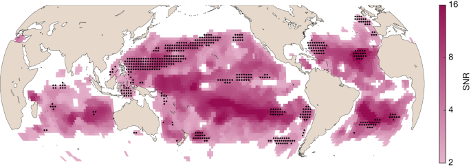
The intensity of the purple colour indicates the SNR. Black stippling indicates regions with significant trends in Chl as well (12% of the ocean). MODIS-Aqua data from July 2002 to June 2022.

We also note that these trends are not associated with changes in sea surface temperature (SST (°C)). When the same analysis is performed for MODIS-Aqua-based SST (Methods), we find significant R_rs trends in 58% of the ocean with a significant SST trend. Because 56% would be expected if R_rs trends were unrelated to SST trends, this suggests that the detected changes in R_rs are not related to changes in SST. Instead, changes in R_rs might be due to other drivers, such as changing mixed-layer depth or upper-ocean stratification²⁹. These drivers are known to affect plankton community structure and biomass, and are expected to change with climate, but are more difficult to detect trends in over shorter time periods (that is, 20 years) than SST because they are measured less precisely.

We thus find that a vast swathe of the ocean has a significant trend in R_rs, when considering many wavebands at the same time. Significant trends tend to occur in low-‘noise’ (that is, weak interannual variability) subtropical and tropical regions, rather than high-‘signal’ regions (Extended Data Fig. 2). The likelihood of SNR exceeding 2 and a trend being detectable increases with decreasing noise levels, but does not increase with increasing signal levels. Significant trends are also neither spectrally narrow (that is, linked to any particular waveband) nor spectrally flat (that is, lacking a spectral signature) (Extended Data Figs. 3 and 4).

Model

A key question is whether the identified trends are driven by climate change. To test this, we performed the same analysis on MODIS-like R_rs data simulated by a numerical model of a complex global ocean ecosystem and associated biogeochemical cycles^2,30. The model simulates the changes to the marine ecosystem and optics over the course of the twenty-first century under a scenario of high greenhouse-gas emissions (Methods). By also considering a control simulation (that is, without perturbation from increased emissions), we can attribute changes to climate change. We analysed this model in terms of the time of emergence (ToE (years))³¹, which quantifies how long it takes for the climate-change-driven trend in a simulation with climate change (that is, a forced simulation) to emerge (with a SNR of 2) from the natural variability in a simulation without climate change (that is, a control simulation), both over the period 2000–2105. For the model R_rs, the ToE is 20 years or less in 46% of the ocean, a comparable fraction to the 56% of the ocean for which we find a significant trend in MODIS-Aqua R_rs (Fig. 2a,b). The (area-weighted) median ToE across the entire model surface ocean is 22 years. By comparison, the ToE is 20 years or less for less than 10% of the ocean for Chl², underscoring that climate-change-driven trends in R_rs can emerge much faster than those for Chl, and on a similar timescale to the observational period investigated here. Given the coarse resolution of the model, it only crudely captures some of the features of the physical circulation in the ocean, such as narrow current systems (for example, the Gulf Stream or equatorial currents). As such, direct comparisons of finer-scale features between model and satellite observations should be done with care. Nonetheless, similar broad regions in both cases are responsible for the significant trends after 20 years, notably the North Atlantic and the subtropical Pacific. Although this is, arguably, the only numerical model suitable for such investigations, which limits the strength of any attribution statement that can be made from it, the consistency in the overall extent and the general location of significant trends in the observations and emerged climate-change-driven trends in the model suggest that the observed trends are indeed driven by climate change. In the model, because changes in community structure emerge much faster than those of Chl or other optically relevant properties, the early emergence of R_rs trends is linked to phytoplankton community structure, which influences food webs, biogeochemical cycles and marine biodiversity.

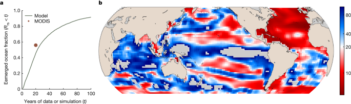
a, Cumulative distribution function of the ToE of the ocean-colour trend in the model simulation. The orange point indicates the fraction of the total surface-ocean area with a significant trend in the 20-year MODIS-Aqua time series. Compare this with Fig. 10 in ref. ², which shows less than 10% of the ocean with an emerged Chl trend after 20 years. b, Map of the ToE in the model simulation (median = 22 years). Grid cells are coloured by percentile, with white at 20 years, such that all white and red grid cells have a ToE of 20 years or less, and all blue grid cells have a ToE of more than 20 years. Grey grid cells do not have significant R_rs trends over the twenty-first century. See ref. ² for a similar plot for Chl.

Discussion

Changes to the surface-ocean ecosystem will affect R_rs (see idealized examples provided in the Supplementary Information). From these considerations, the changes in R_rs and the spatial patterns seen in Extended Data Fig. 3 are complex, likely to be multifaceted and defy simple description. In the broadest terms, increases in R_rs are more frequent than decreases, and increasingly so for intermediate wavelengths, suggesting that the ocean is on the whole becoming greener. This greening could result for instance from an increase in detrital particles, which would increase backscattering at all wavelengths and absorption at shorter wavelengths. However, it could also result from other possible ecosystem shifts, such as a simultaneous increase in zooplankton and coloured dissolved material. Nonetheless, and regardless of any comparison with model trends, the observed changes in R_rs will necessarily have ecological implications. Irrespective of which optical constituent(s) in the surface ecosystem changed to produce a trend in R_rs, any such optical change will alter the light environment. Because light is a key driver of phytoplankton communities, any change in the light environment—whether due to changes in in-water optical constituents or changes in light availability entering the ocean—will lead to a change in the surface-ocean ecosystem.

Altogether, these results suggest that the effects of climate change are already being felt in surface marine microbial ecosystems, but have not yet been detected because previous studies have considered Chl or other univariate approaches. R_rs facilitates the early detection of climate-change signals by integrating, and being sensitive to, changes in the properties of surface-ocean ecosystems. R_rs, and thus surface-ocean ecology, has changed significantly over a large fraction of the ocean in the past 20 years. The changes in R_rs that we have identified have potential implications both for the role of plankton in marine biogeochemical cycles and thus ocean carbon storage, and for plankton consumption by higher trophic levels and thus fisheries. Our findings therefore might be of relevance for ocean conservation and governance. For instance, knowledge of where the surface-ocean microbial ecosystem is changing might be useful for identifying regions of the open ocean in which to establish marine protected areas under the United Nations high seas treaty on the biodiversity of areas beyond national jurisdiction. The identified locations with changes in R_rs are consistent with where changes are expected in drivers such as upper-ocean stratification, but might be more easily detectable on the global scale—as we have done here—thanks to the multivariate and low-interannual-variability nature of R_rs. This highlights the value of long-term satellite missions like MODIS-Aqua and of space agencies maintaining missions for as long as is feasible. That significant trends occur primarily where interannual variability is low means that a similar signal may be expected to emerge in other portions of the ocean in coming years, although the MODIS-Aqua mission is scheduled to end in the near future. Thus for future work, merged multi-satellite products, as well as work that is currently underway to improve them, are essential. Ongoing work³² interpreting R_rs could shed light on what the trends found here indicate about precisely how surface-ocean ecology is changing^33,34; we hope that the results presented here will spur further work to this end. Given the key role of plankton ecosystems in marine food webs, global biogeochemical cycles and carbon cycle–climate feedbacks, detecting change in these ecosystems is of great utility.