


We first analyse how rates of friendship formation, EC, exposure and friending bias vary across settings.
Figure 1 shows how the share of friends that an individual makes in each setting varies with their SES rank. For each SES ventile, it plots the average proportion of friends made in each setting, divided by the overall proportion of friends made in that setting across all SES ventiles. Individuals with the lowest SES make about four times greater a share of their friends in their neighbourhoods (residential ZIP codes) compared with individuals with the highest SES. By contrast, high-SES individuals make a far greater share of their friends in college than low-SES individuals do, primarily because individuals with high SES are much more likely to attend college. Neighbourhoods therefore play a larger role in defining the social communities of low-SES individuals, perhaps explaining why where one lives matters more for the economic and health outcomes of lower-income individuals than higher-income individuals22,23.
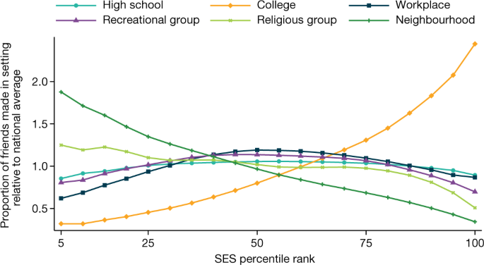
Friending rates across settings by the SES percentile rank of individuals in our primary analysis sample. The primary analysis sample consists of individuals between the ages of 25 and 44 years as of 28 May 2022 who reside in the United States, have been active on the Facebook platform at least once in the previous 30 days, have at least 100 US-based Facebook friends, have a non-missing residential ZIP code and for whom we are able to allocate at least one friend to a setting using the algorithm described in the ‘Variable definitions’ section of Methods. The vertical axis shows the relative share of friends made in each of the six settings that we analyse (for example, high schools), defined as the average fraction of friends made in that setting by people in a given SES ventile (5 percentile rank bin) divided by the fraction of friends made in that setting in the whole sample. Numbers above 1 imply that people at a given SES rank make more friends in a given setting than the average person; numbers below 1 imply the opposite. Extended Data Table 4 lists the underlying shares of friendships made in each setting for people with below-median SES versus above-median SES.
Figure 2a shows how EC varies across the six settings for people with below- versus above-median SES. For each SES category, we define the setting-specific EC as two times the average share of friends made in that setting who have high SES. EC for people with low SES is highest in colleges and lowest in their residential neighbourhoods. However, even in colleges, low-SES people are much less likely to befriend high-SES people than high-SES people are. To understand why, we next examine rates of high-SES exposure and friending bias in each setting.
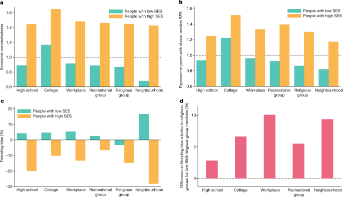
a–d, Variation in EC, exposure and friending bias across six settings where friendships are formed by individuals’ SES. All of the plots are based on the primary analysis sample defined in the legend of Fig. 1. a, Economic connectedness (EC) by setting for individuals with below-median SES (left, green bars) and above-median SES (right, orange bars). For both low- and high-SES individuals, EC is defined as twice the fraction of above-median-SES friends made within each setting. b, Mean rate of exposure to high-SES individuals in an individual’s group (for example, their high school) by setting for individuals with below-median SES (left, green bars) and above-median SES (right, orange bars). High-SES exposure is defined as two times the fraction of above-median-SES members of the individual’s group. c, Mean friending bias by setting for individuals with below-median SES (left, green bars) and above-median SES (right, orange bars). Friending bias is defined as one minus the ratio of the share of above-median-SES friends to the share of above-median-SES peers in the individual’s group. EC, high-SES exposure and friending bias are all calculated at the individual level and then aggregated to the setting × SES level (Supplementary Information B.5). d, Restricting the sample to low-SES members of religious groups, plots these individuals’ friending bias in each of the other settings minus their friending bias in religious groups. Extended Data Table 4 lists the values of average EC, bias and exposure shown in this figure.
Figure 2b shows average exposure to high-SES peers for low- and high-SES individuals across the six settings, among those who are assigned to a group in that setting. The exposure of individuals with low SES to high-SES peers is below 1 (that is, fewer than 50% of their peers have above-median SES) on average in all settings except in colleges, in which exposure is above 1 because most people who attend college have high SES. By contrast, for individuals with high SES, exposure to high-SES peers is well above 1 in all settings. This disparity in exposure reflects segregation across groups; for example, high-SES people tend to attend different religious institutions and colleges compared with low-SES people, as is well known from previous studies on segregation.
Social network data enable us to go beyond measures of segregation and analyse differences in rates of interaction conditional on exposure. This ability to identify interaction (friendship) rather than merely exposure (geographical proximity) is a key distinction between the present study and recent work that measures experienced segregation using location data from mobile devices24,25,26,27,28. Figure 2c shows mean rates of friending bias—the extent to which rates of friendship with high-SES individuals deviate from rates of exposure to high-SES individuals—across settings. The green bars show that levels of friending bias for individuals with low SES are typically positive, but differ substantially across settings.
Friending bias is highest on average in neighbourhoods, in which the mean friending bias for individuals with low SES is 0.17. That is, low-SES people befriend high-SES people in their ZIP codes at a 17% lower rate than would be the case if they were to befriend individuals with high SES in proportion to their presence in their ZIP codes. Friending bias may be high at the neighbourhood level partly because of residential segregation within ZIP codes that limits opportunities for contact and interaction between people with low and high SES.
Friending bias is lowest on average in religious groups, in which friending bias is −0.03, implying that low-SES people tend to form friendships with high-SES members of their religious groups at a rate that is slightly higher than the share of high-SES people in their religious groups. Friending bias is negative in religious groups because religious-group friendships do not exhibit substantial homophily by SES—a finding that is consistent with previous research using survey data29—and because high-SES people make more friends than low-SES people. Holding fixed exposure, people with low SES are about 20% more likely to befriend a given high-SES person in their religious groups than in their neighbourhoods—a large difference, comparable in magnitude to the 22.4% under-representation of high-SES friends on average among low-SES individuals7. Put differently, if friending bias in all settings was reduced by an amount equal to the difference in friending bias between neighbourhoods and religious groups, most of the disconnection between low-SES and high-SES individuals in the US would be eliminated.
Since religious groups are highly segregated by income, as shown in Fig. 2b, their low friending bias does not currently translate to a high level of EC (Fig. 2a). Efforts to integrate religious groups by SES may be particularly effective at increasing EC if friending bias remains low as they become more integrated. This assumption is not innocuous—as illustrated by the challenges faced in efforts to integrate college classrooms30—but it is bolstered by the fact that religious groups exhibit low levels of friending bias at all levels of exposure (Supplementary Fig. 1b).
Figure 2c (orange bars) shows that, across all settings, people with high SES are more likely to befriend their fellow high-SES group members (and correspondingly less likely to befriend low-SES group members) than would be expected based solely on the socioeconomic compositions of their groups. Again, there is sizable heterogeneity in friending bias across settings: high-SES people exhibit the most friending bias (in absolute terms) in neighbourhoods, and the least in recreational groups.
A natural question that arises from these differences in friending bias across settings is whether they are an attribute of the setting itself, or a reflection of the types of individuals who join that setting. For example, religious groups might be particularly good at fostering ties between low- and high-SES members, or it could be that individuals who participate in religious groups are more likely to form cross-SES ties across all settings. To distinguish between these explanations, Fig. 2d plots friending bias in each of the other five settings minus friending bias in religious groups for low-SES members of religious groups. Members of religious groups exhibit much more friending bias in all other settings than they do in religious groups, showing that the settings in which friendships form matter.
The fact that friending bias varies significantly across settings suggests that it is in substantial part determined by the nature of the institutions in which people interact—consistent with Blau’s theory of social structure31—rather than entirely determined by preferences. This result suggests that friending bias can potentially be changed through policy interventions (for example, by changing the structure of the groups in which people interact), much as the socioeconomic composition of groups can be influenced by policy (for example, through busing or affordable housing programs). Next, we analyse how important it is to reduce friending bias versus increase exposure to increase EC by examining the relative contributions of these factors in generating differences in connectedness.
Decomposing connectedness by SES
We quantify how much of the difference in the share of high-SES friends between people with low versus high SES is due to differences in friending shares across settings, differences in exposure, and differences in friending bias by conducting counterfactual exercises that sequentially remove variation in each of these three dimensions (Methods: ‘Decomposing EC’). Conceptually, our goal is to determine how much of the difference in connectedness would remain if people with low SES made friends in different settings at the same rates as high-SES people (same friending shares); if they participated in groups with the same shares of high-SES members (same exposure); and if they made friends with high-SES peers at the same rates conditional on exposure as high-SES individuals do (same friending bias).
Figure 3a presents the results of this exercise. The top bar shows that EC for the average low-SES individual is 0.83, whereas the bottom bar shows that EC for the average high-SES individual is 1.53—corresponding to a gap in EC by SES of 0.7 (Methods: ‘Decomposing EC’). Now consider equating the share of friends that the average low-SES person makes across the six settings to match that of the average high-SES person. Intuitively, this exercise examines what would happen to the EC of low-SES people if they were to make friends at the same relative rates across settings as high-SES people holding constant rates of exposure and friending bias across settings. For example, this counterfactual would increase the overall share of friends that low-SES people make in college to match that of high-SES people; however, it would not change the specific colleges that low-SES people attend to match those of high-SES people (as changes in groups within settings would generate a change in exposure).
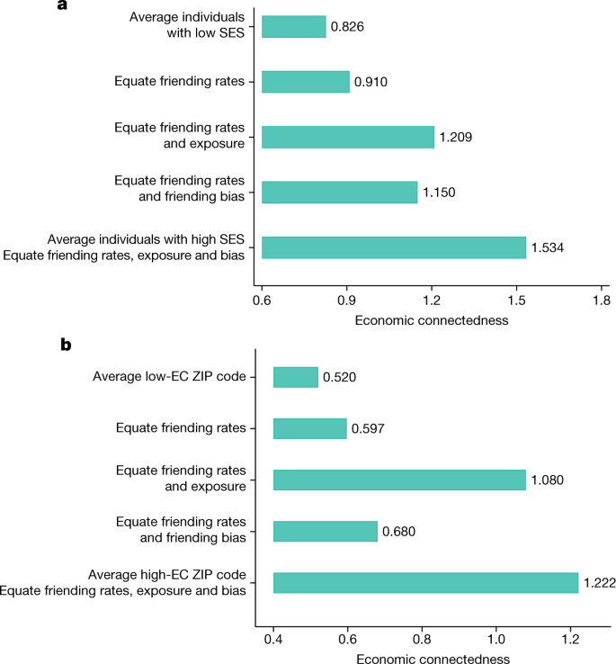
a, Share of the difference in EC between individuals with high versus low SES that is driven by differences in the settings in which they make friendships (friending rates), rates of exposure to individuals with high SES in those settings and friending bias conditional on exposure. The first and fifth bars show the observed EC for average low- and high-SES individuals, calculated as the EC for individuals who have setting-level friending rates, exposure rates and friending bias levels that match the means for low- and high-SES people in our sample, respectively (Methods: ‘Decomposing EC’). The middle three bars show the predicted EC for the average low-SES individual under various counterfactual scenarios. In the second bar, we consider a counterfactual scenario in which the friending rates across different settings for the average low-SES individual are equated to those of the average high-SES individual, while preserving exposure and friending bias at the mean observed levels for low-SES individuals within those settings. The third bar further equates the rate of high-SES exposure in each setting to match the observed mean values for high-SES individuals. The fourth bar equates rates of friending bias in each setting as well as friending rates across settings to match the observed mean values for high-SES individuals. The fifth bar equates rates of both exposure and friending bias within settings and friending rates across settings. b, A decomposition exercise analogous to a between ZIP codes with different levels of EC for below-median-SES residents instead of between individuals with below- versus above-median SES. The comparison of interest here is between ZIP codes in the bottom quintile of the EC distribution for below-median-SES residents (low-EC ZIP codes) and ZIP codes in the top quintile of EC for below-median-SES residents (high-EC ZIP codes). See Supplementary Information B.5 for further details on these counterfactual exercises.
The second bar in Fig. 3a shows that equating friending shares across settings by SES closes only 12% of the gap in EC between the average person with low versus high SES. Thus, differences in the settings in which people make friends explain little of why high-SES people have more high-SES friends. This is consistent with the fact that the variation in EC across settings for individuals with low SES is small compared with differences in EC by SES within each setting (Fig. 2a): even if low-SES individuals were to make all their friends in their highest-EC setting (colleges), their EC would still be substantially below that of high-SES individuals.
Next, we preserve these equated friend shares across settings and set the exposure rates in each setting for the average low-SES person to match the exposure rate for the average high-SES person in that setting. This counterfactual resembles a desegregation policy that adjusts the socioeconomic composition of groups but leaves friendship patterns within them unchanged. For example, in the context of colleges, this counterfactual can be interpreted as having students with low SES attend the same colleges as students with high SES, but retaining their current rate of befriending a given high-SES college peer. The third bar in Fig. 3a shows that equating exposure in addition to friending shares would increase the EC of the average low-SES individual to 1.21, closing 54% of the gap in EC between the average person with low versus high SES. Intuitively, this is because the gap in exposure by SES in Fig. 2b is approximately half as large as the gap in EC in Fig. 2a in most groups. Although a 54% reduction is substantial, it implies that even if neighbourhoods (ZIP codes), schools and colleges were perfectly integrated by SES, nearly half of the gap in EC between individuals with low and high SES would remain.
In the fifth bar, we further set friending bias in each setting for the average low-SES person equal to friending bias of the average high-SES person in that setting. Equating friending bias mechanically closes the remaining 46% gap in EC between the average person with low versus high SES.
Decomposing connectedness across areas
We use a similar approach to analyse why EC among people with low SES varies geographically7. We begin by collapsing our individual-level measures of exposure and bias to the county level, calculating mean high-SES exposure and friending bias among individuals with low SES for each county. Figure 4 maps these variables by county. Furthermore, we provide an illustrative example of local-area variation by presenting maps of these variables by ZIP code in the Los Angeles metropolitan area. As one might expect, exposure is generally higher in places with higher average incomes (Supplementary Information C.2), such as along each coast of the continental United States and near the coast in Los Angeles. Friending bias is lowest in the Midwest and Great Plains. Friending bias is lower on average in areas with more high-SES exposure, with a correlation of about −0.2 across counties, but there are many exceptions to this pattern. For example, the northeast generally has high exposure but also high friending bias (that is, people with low and high SES in the northeast are relatively well integrated in schools and neighbourhoods, but tend to befriend each other at lower rates).
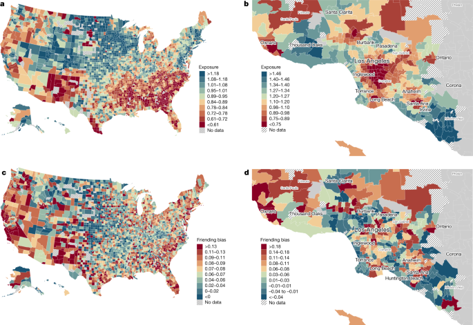
a–d, Maps of mean high-SES exposure (a,b) and mean friending bias (c,d) for individuals with low SES. a,c, National county-level maps. b,d, ZIP-code-level maps of the Los Angeles metropolitan area. We aggregate individual-level statistics to compute ZIP-code-level and county-level means (Supplementary Information B.5). At the individual level, exposure is defined as the weighted average of two times the fraction of individuals with above-median SES in the groups in which an individual with below-median SES participates, weighting each group by the individual’s share of friends in that group. Friending bias is defined as one minus the weighted average of the ratio of the share of high-SES friends to the share of high-SES peers in the groups in which an individual with low SES participates, again weighting each group by the individual’s share of friends in that group. We use methods from the differential privacy literature to add noise to the statistics plotted here to protect privacy while maintaining a high level of statistical reliability; see www.socialcapital.org for further details on these procedures.
We use these area-level statistics to decompose the sources of the ZIP-code-level variation in the EC of individuals with low SES (Methods: ‘Decomposing EC’). The top bar in Fig. 3b shows that the average EC for people with low SES living in ZIP codes that are in the bottom quintile of the national distribution of ZIP-code-level low-SES EC averages is 0.52. The bottom bar shows that the corresponding value for people with low SES living in the top quintile of ZIP codes (again in terms of average levels of EC among individuals with low SES) is 1.22. The bars in the middle decompose this top-to-bottom-quintile difference in EC by sequentially equating the share of friends made in different settings, rates of exposure to high-SES peers and rates of friending bias of the average low-SES person in bottom-EC-quintile ZIP codes to match the corresponding values for the average low-SES person in top-EC-quintile ZIP codes (Supplementary Information B.5). We find that 73% of the difference in EC between ZIP codes in the bottom and top quintiles of the EC distribution is explained by differences in exposure, while 16% is explained by differences in friending bias and 11% by differences in friending rates across settings.
The geographical variation in EC is driven primarily by differences in exposure because high SES exposure varies more at the geographical level, whereas friending bias varies more across settings (for example, between neighbourhoods and religious groups). The variation in exposure is 3.3 times greater across counties than across settings (Extended Data Table 1). By contrast, the variation in friending bias is 3.3 times greater across settings than across counties. Intuitively, in areas in which the share of people with high SES is high in one setting (for example, in neighbourhoods), it is generally high in other settings as well (for example, in schools). By contrast, friending bias tends to be relatively consistent by setting across geographies, with low-bias settings in one area (for example, religious groups) generally exhibiting low friending bias in other areas as well. In short, where one lives influences one’s exposure to individuals with high SES, but the groups in which one participates substantially shape the extent to which one interacts with those high-SES peers.
In summary, differences in high-SES exposure generate most of the variation in the EC of people with low SES across areas, but friending bias and exposure contribute about equally to explaining the difference in the share of high-SES friends between low- and high-SES people. The reason is that exposure varies more across areas than it does by individual socioeconomic status, whereas friending bias differs sharply by SES and is relatively stable (but large) across areas.
Exposure, bias and upward mobility
Given that both exposure and friending bias contribute to differences in EC, we next examine whether the strong correlation between EC and upward income mobility documented in the companion paper7 is driven by one or both of these components. We define upward mobility as the average income rank in adulthood of children who grew up in families at the 25th percentile of the national income distribution in a given county or zip code, drawing on data from the Opportunity Atlas23.
In column 1 of Table 1, we regress log[upward mobility] on log[EC] across ZIP codes (Methods: ‘Exposure, bias and upward mobility’). We find an elasticity of upward mobility with respect to EC of 0.24: a 10% increase in EC is associated with a 2.4% increase in upward mobility. In column 2, we regress log[upward mobility] on log[exposure] and log[1 − friending bias]. We find strong associations between both exposure and friending bias and measures of upward mobility, with elasticities of 0.25 and 0.19, respectively. Next, we examine how these relationships vary within versus across counties. Columns 3 and 4 of Table 1 include county fixed effects in the specifications from columns 1 and 2. When comparing ZIP codes within counties, higher exposure and lower friending bias remain strongly associated with higher levels of economic mobility, with elasticities of just under 0.25. In columns 5 and 6, we conversely focus on across-county variation by replicating columns 1 and 2 at the county level. We find qualitatively similar effects, although the estimates of the effects of friending bias on economic mobility become less precise, largely because most of the variation in friending bias is within rather than across counties (Extended Data Table 1).
In column 7 of Table 1, we change the dependent variable in the regression to the log of each county’s causal effect on upward mobility as estimated by Chetty and Hendren based on analysing movers32 (see the companion paper7 for further details on the interpretation of these causal effect measures). Both exposure and friending bias remain strongly predictive of counties’ causal effects on upward mobility, implying that moving to a place with greater exposure or lower friending bias at an earlier age increases the earnings in adulthood of children who grow up in low-income families.
We conclude that the relationship between economic connectedness and upward mobility is not driven merely by the presence of high-SES peers (for example, through the availability of additional resources for schools financed by local property taxes). Instead, interaction with those peers is what predicts upward mobility most strongly (see Supplementary Information C.3 for further discussion). In the context of schools, this result implies that the average income of classmates predicts upward mobility for low-SES students insofar as it affects the extent of their social interactions with high-SES students. Combined with our finding that friending bias accounts for around half of the difference in the share of high-SES friends between people with low versus high SES, these results imply that increasing EC—the form of social capital most strongly associated with economic mobility—would require efforts to both increase integration (exposure) and reduce friending bias within groups. In the next section, we show how our data can inform which of these approaches is likely to be most effective in a given group.
Exposure and friending bias by high school
Having shown how exposure and friending bias vary across settings and areas, we now analyse variation in these statistics across the groups that comprise a given setting (for example, each high school in the ‘high school’ category). We begin by examining variation across high schools and then turn to variation across colleges. We publicly release estimates of exposure and friending bias for each high school and college as well as by neighbourhood (ZIP code); for religious organizations, recreational groups and employers, sample sizes are too small to obtain reliable estimates at the group-specific level.
For high schools, we report estimates based both on students’ own (post-high-school) SES in adulthood—the same SES measure that was analysed above—as well as estimates based on their parents’ SES (Methods: ‘High school estimates’). These measures have different applications. Measures of EC based on parental SES are relevant for policy discussions at the school level, which often focus on the degree of connection between children from different parental backgrounds. Measures based on own SES are useful for understanding the environments in which friendships between low-SES and high-SES adults are formed, that is, the extent to which a school might contribute to levels of EC in the next generation. Although the two measures capture different concepts, they yield fairly similar rankings of schools in terms of exposure and friending bias: the correlation between the two measures is 0.84 for exposure and 0.59 for friending bias across schools (Supplementary Table 1). We therefore focus on the parental SES measure here and present analogous results using own SES in Supplementary Fig. 2.
Figure 5a plots friending bias (with an inverted vertical scale, so that moving up corresponds to less bias) against the share of students with high parental SES (that is, half of high-SES exposure) by high school. Both exposure to students with high parental SES (socioeconomic composition) and friending bias vary substantially across schools. The reliability of the exposure estimates, estimated using a split-sample approach (Methods: ‘High school estimates’), is 0.99 at the school level; that is, 99% of the variance in exposure reflects true differences in the share of students with high parental SES rather than sampling error. The reliability of the friending bias estimates is 0.58. This implies that a school that we estimate to have a 10% higher friending bias estimate will, on average, exhibit 5.8% higher bias in future cohorts. Estimates of exposure and friending bias based on own SES have higher reliabilities (0.99 for exposure and 0.88 for friending bias) because they use the full sample rather than just the subset of individuals that we can link to their parents.
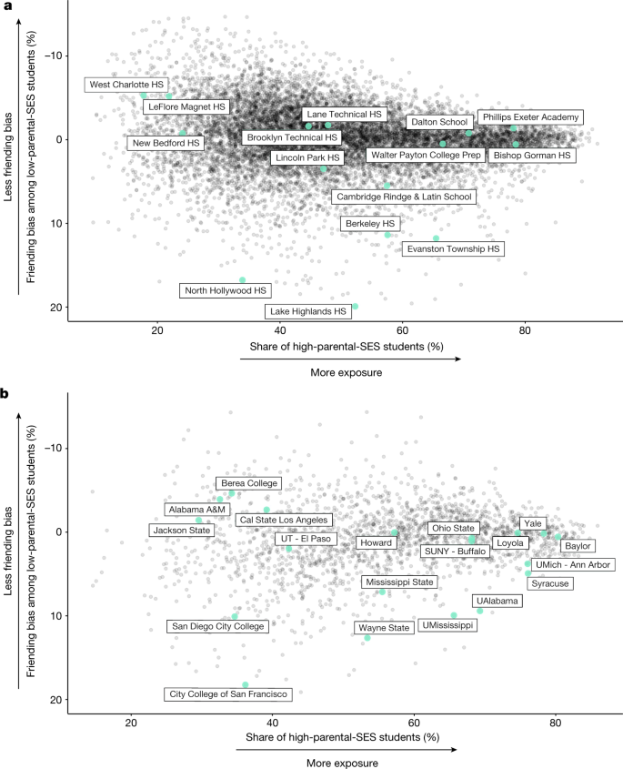
a,b, Mean friending bias among students with low parental SES versus the share of students with high parental SES by high school (a) and college (b). Friending bias is defined as one minus the mean ratio of the share of high-school friends with high parental SES to the share of high-school peers with high parental SES, averaging over students with low parental SES (Supplementary Information B.5).The vertical axis is reversed, so that schools and colleges in the upper half of each panel have lower friending bias. The sample consists of individuals in the 1990–2000 birth cohorts (approximately spanning the high school and college graduating classes of 2008–2018 and 2012–2022, respectively) who could be linked to a specific school or college and to parents with an SES prediction. We report statistics only for high schools and colleges that have at least 100 low-SES and 100 high-SES Facebook users summing across these cohorts. We use methods from the differential privacy literature to add noise to the statistics plotted here to protect privacy while maintaining a high level of statistical reliability; see https://www.socialcapital.org for further details on these procedures. In this figure, SES refers to the SES of the individuals’ parents; Supplementary Fig. 2 replicates these figures using individuals’ own (post-high school and post-college) SES ranks in adulthood.
Friending bias differs considerably even among nearby schools with similar socioeconomic compositions. For example, Walter Payton College Preparatory High School (‘Payton’) and Evanston Township High School (‘ETHS’) are two large high schools in the Chicago metro area that have similar fractions of students from families with above-median SES. However, ETHS has much higher friending bias than Payton: low-SES students at ETHS are much less likely to befriend their high-SES peers than low-SES students at Payton are, consistent with previous ethnographic evidence documenting high levels of friending bias at ETHS (Supplementary Information C.4). One potential explanation for this difference is the greater similarity of students on other dimensions at Payton relative to ETHS. Payton is a public magnet school that requires that all students complete an entrance exam. By contrast, ETHS is open to all students residing in the local catchment area, resulting in a more heterogeneous student body in terms of academic preparation—and concomitant segregation of classes—that may lead to higher friending bias33.
Predictors of friending bias
Building on this comparison, we examine the factors that predict friending bias across high schools more systematically by correlating bias across schools with various observable characteristics. Consistent with the ETHS–Payton comparison, we find that friending bias is higher on average in schools with more academic tracking as measured by enrolment rates in advanced placement and gifted and talented classes (Extended Data Fig. 1a,b). Friending bias is generally lower in smaller schools (Extended Data Fig. 1c), consistent with previous work documenting less homophily in smaller groups31,34,35.
In Extended Data Fig. 1d, we examine the relationship between friending bias and a school’s share of students with high parental SES. This relationship is non-monotonic, with friending bias highest in schools with an approximately equal representation of students from families with below- and above-median SES. This may be because there is less scope for low-SES or high-SES students to develop homogeneous cliques when there are relatively few members of their own group. Friending bias is also higher in more racially diverse schools, as measured by a Herfindahl–Hirschman index (Extended Data Fig. 1e) or the share of white students in the school (Extended Data Fig. 1f). One potential explanation for the link between racial diversity and friending bias by SES is that, when low- and high-SES students have different racial and ethnic backgrounds, they are less likely to be friends.
There are similar associations between these factors and friending bias between students who go on to have different socioeconomic statuses in adulthood themselves (Extended Data Fig. 2). In particular, in smaller and less racially diverse schools, there are more friendships between students who go on to have low and high SES in adulthood. We also find similar relationships between friending bias and group characteristics in other settings: higher levels of friending bias are associated with greater racial diversity across colleges and neighbourhoods (Extended Data Fig. 3) and larger group sizes across all six settings (Supplementary Fig. 1).
The explanatory factors considered in Extended Data Figs. 1–3 are not intended to be exhaustive, and much more remains to be learned about the determinants of friending bias. The main lesson we draw from these correlations is that, much like exposure, friending bias appears to be related to structural factors that can potentially be changed by policy interventions, such as reducing the size of groups and redesigning the nature of academic tracking within schools.
Increasing connectedness
The variation in exposure and friending bias across schools documented in Fig. 5a implies that the most effective approach to increasing EC differs across schools. To increase EC in schools in the bottom half of Fig. 5a—such as Evanston Township High School, Berkeley High in Berkeley, CA, or Lake Highlands High in Lake Highlands, TX—decreasing friending bias (that is, increasing social interaction between students from different backgrounds) is likely to be valuable. For example, reducing friending bias at ETHS to zero would result in an increase of 0.15 (15 percentage points) in EC (measured in terms of parental SES). To benchmark this impact, note that the average parental EC among high school friends of individuals with low-SES parents across the schools in Fig. 5a is 0.92. This implies that, in the average US high school, students with low parental SES have 8% fewer high-parental-SES friends than one would expect in a scenario where students with high and low SES made the same total number of high school friends and exhibit no homophily. The current level of friending bias at ETHS therefore reduces the share of high-SES friends among low-SES students by almost twice the degree of under-representation of high-SES friends among students from low-SES families at the average US high school (15% versus 8%). Thus, at schools like ETHS, increasing cross-SES interaction within the student body may be a more effective way to increase EC than attempting to further diversify the student body. By contrast, for schools that exhibit low levels of exposure and low levels of bias, such as West Charlotte High or LeFlore Magnet (shown in the top left quadrant of Fig. 5a), increasing socioeconomic integration (exposure) is a necessary first step to increasing EC.
The preceding analysis focuses on how to maximize EC from the perspective of a given student with low SES (that is, how to increase the likelihood that they form cross-SES friendships within a given school). However, from a social perspective, it may be more relevant to consider a given school’s contribution to the total number of cross-SES friendships in society. To see how these concepts differ, consider Phillips Exeter Academy, an elite private school in New Hampshire where almost 80% of students come from families with above-median SES (exposure is high) and friending bias is low (below zero). Given these conditions, Phillips Exeter students with low SES tend to form many friendships with their high-SES classmates and have a high EC. However, because students with low SES make up only a small share of Phillips Exeter’s students, the total number of cross-SES connections that Phillips Exeter generates is relatively small. If Phillips Exeter were to enrol more students with low SES (and fewer with high SES), it could increase its total contribution to connectedness despite reducing EC for current low-SES students (as they would be exposed to fewer high-SES peers).
We measure each school’s total contribution to EC (TCEC) as the product of the share of low-SES students and the average EC among low-SES students in that school (Methods: ‘Total contribution to connectedness’). TCEC measures how many friendships a school creates between students with high and low SES, holding fixed total enrolment and the total number of friends that students make across schools. Reducing friending bias at a school (all else equal) always increases the total number of friendships between students with low and high SES. However, increasing the share of high-SES students has non-monotonic effects on TCEC. Schools that have very few high-SES students offer few opportunities for their low-SES students to meet high-SES peers and therefore contribute little to overall economic connectedness. Conversely, schools that have predominantly high-SES students, such as Phillips Exeter or the Dalton School in New York City, provide many high-SES connections to the low-SES students that they do enrol, but offer those opportunities to relatively few low-SES students and therefore also have low TCEC.
Owing to these competing forces, when holding friending bias fixed, an above-median-SES share of 50% (that is, achieving perfect socioeconomic integration) maximizes the total number of cross-class connections at a school. Schools that have low friending bias and near-equal representation of students with below- and above-median parental SES—such as Lane Technical in Fig. 5a—contribute the most to total EC in an accounting sense. More generally, the direction in which one must shift exposure to increase the total number of cross-SES links differs on the basis of a school’s initial share of high-SES students. By contrast, reducing friending bias always increases EC for a given low-SES student as well as TCEC.
Furthermore, increasing the share of high-SES students in one school necessarily requires reducing the share of high-SES students in at least one other school, as the total number of students with above-median SES is fixed. As a result, increasing high-SES shares even at schools where high-SES shares are below 50% can have ambiguous effects on EC in society as a whole. If the high-SES students who join a given school A otherwise would have attended school B where they would have connected with more low-SES peers, overall EC in society could fall even though TCEC at school A would rise. Thus, one must be cognizant of the counterfactual distribution of SES across schools when evaluating the effects of increasing exposure. By contrast, efforts to reduce friending bias in a given school do not generally have direct implications for connectedness at other schools.
In summary, for schools that already have diverse student bodies (that is, schools that have a balanced socioeconomic representation) but high levels of friending bias, initiatives to identify and address institutional factors contributing to friending bias may be the most fruitful path to increasing their total contributions to connectedness. For schools that currently have less diverse student bodies, it may be valuable to increase diversity in a manner that takes account of which schools the new students would otherwise have attended.
Exposure and friending bias by college
Figure 5b replicates Fig. 5a for colleges, again using parental SES. We see analogous heterogeneity in exposure and friending bias across colleges, with similar implications. For example, Yale University exhibits relatively low friending bias and has a large high-SES share, resulting in high levels of EC for its low-SES students. However, because students with low SES make up only a small share of the student body, Yale, similar to many other elite private colleges, creates relatively few cross-SES connections (it has low TCEC).
Among colleges with more socioeconomically diverse student bodies, such as Wayne State and Howard, there is again considerable variation in connectedness that results from differences in friending bias. Similar to high schools, friending bias tends to increase with a college’s size and with the degree of racial diversity of the student body (Supplementary Fig. 3). In a different vein, ethnographic evidence suggests that many colleges that exhibit high levels of bias—such as the University of Alabama, Syracuse University, or the University of Mississippi—feature significant Greek life, where the high costs of fraternity and sorority dues may generate friending bias on campus36. Similarly, community colleges without a substantial residential student population (for example, the City College of San Francisco or San Diego City College) tend to exhibit high levels of friending bias. Systematically evaluating these and other hypotheses using the data constructed here would be a useful direction for further work. For now, these results again suggest that friending bias is at least partly determined by structural factors that could potentially be changed by colleges, much like recent efforts to increase socioeconomic diversity at elite private colleges.
Effects of integration on connectedness
Having established that there is significant variation across schools and colleges in friending bias and exposure, we now examine whether these estimates are sufficiently reliable to determine what interventions will be most effective at increasing EC in a given school. As a practical illustration, consider policies that seek to increase socioeconomic diversity in a given school district. We examine whether our estimates of average friending bias can be used to reliably identify the schools in which such policies will increase connectedness the most. If estimates of friending bias are perfectly stable, the effect of a change in socioeconomic composition will be well predicted by historical estimates of average friending bias. By contrast, if estimates of bias change over time (for example, due to measurement error or drift), or if the effects of incremental changes in socioeconomic diversity on EC differ substantially from historical averages of friending bias, predictions based on existing observational data may not provide reliable forecasts. It is therefore an empirical question whether the school-level estimates that we report provide useful information to predict the effects of policy changes. We use two quasi-experimental research designs to identify the causal effects of changes in exposure on connectedness—cross-cohort fluctuations and regression discontinuity—and show that our school-level estimates of average friending bias predict the causal effects of these changes in exposure on economic connectedness.
Cross-cohort fluctuations
In our first approach, we analyse the effects of fluctuations in the share of students with high SES across cohorts within a high school on students’ friendship patterns. Such fluctuations in cohort composition are largely a consequence of random variation in the student body, as discussed in the ‘Cross-cohort fluctuations’ section of the Methods. Intuitively, we compare low-SES students who attend the same school and examine whether those who happen to be in cohorts that have a larger share of high-SES students tend to have more high-SES friends as a result. To harness more variation across cohorts, we focus here on connections between individuals with parents in the lowest and highest SES quintiles (rather than below- versus above-median SES, as we do in the rest of the paper).
Figure 6a presents a binned scatter plot of changes in EC for low-SES students across cohorts within a school versus cross-cohort changes in high-SES exposure (Methods: ‘Cross-cohort fluctuations’). In this analysis, we focus on measuring within-cohort EC and exposure—that is, the shares of high-SES friends and peers that low-SES students have within only their own cohorts in their high schools. The strong positive relationship demonstrates that, within a given school, students in cohorts that happen to have more high-SES students have significantly more high-SES friends in their cohorts on average. Thus, greater high-SES exposure translates to a significantly greater number of high-SES friendships on average, showing that socioeconomic integration can be a powerful tool for increasing cross-class interaction.
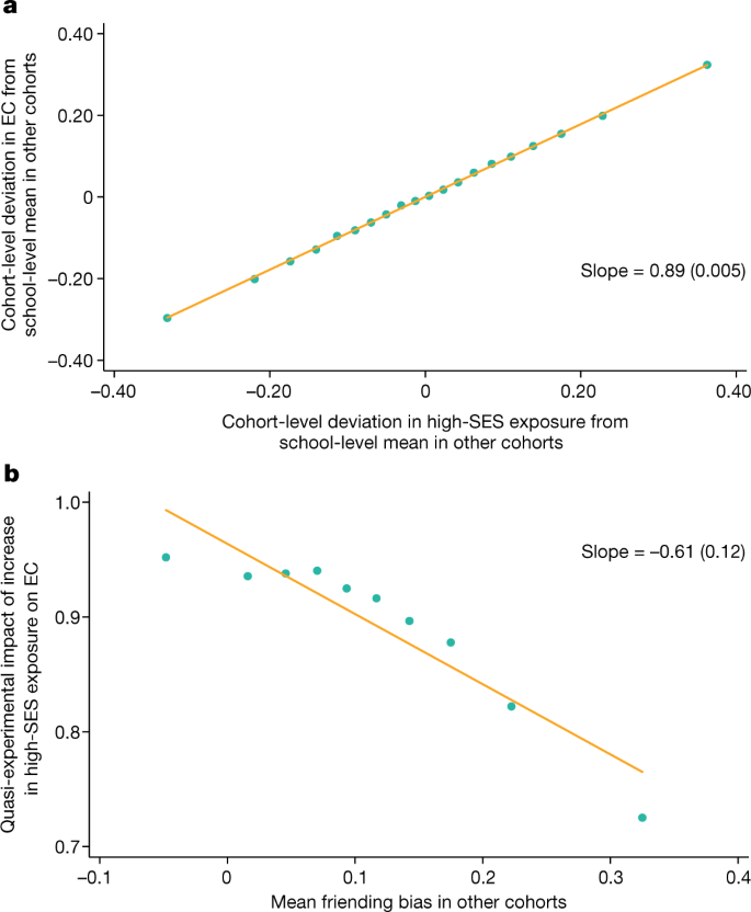
a,b, Analysis of the causal effect of being assigned to a high school cohort with more high-SES peers on the EC of low-SES students, based on the level of friending bias in the school (Methods: ‘Cross-cohort estimates’). a, Cohort-level changes in economic connectedness of low-SES students versus changes in the share of high-SES students. b, Causal impacts of high-SES share on economic connectedness of low-SES students, by level of friending bias. We measure EC, exposure and bias in this figure based on parental SES. The sample consists of all of the individuals in our primary analysis sample who were born between 1990 and 2000 whom we can link to parents and match to high schools. We further limit the sample to schools with at least 500 students (pooling all cohorts), at least 100 bottom-quintile-SES students and at least 100 top-quintile-SES students. For each cohort, exposure is defined as five times the fraction of top-quintile-SES students. EC in a cohort is defined as five times the average share of top-quintile-SES friends among bottom-quintile-SES students. Friending bias is defined as the average among bottom-quintile-SES students of one minus the ratio of the share of friends with top-quintile SES to the share of peers with a top-quintile SES in their cohort. In a, a binned scatter plot is shown of the cohort-level deviations from school means in EC versus cohort-level deviations from school means in exposure. The cohort-level deviations are constructed as the mean for the relevant cohort c in a given school minus the mean for all other cohorts in the same school, weighting by the number of students with bottom-quintile SES in each cohort. The binned scatter plot is constructed by dividing the cohort-level deviations in exposure into 20 equally sized bins and plotting the mean deviation in EC versus the mean deviation in exposure within each bin. We also report a slope estimated using a linear regression, with standard error clustered by high school in parentheses. To construct the plot in b, we first divide school × cohort cells into deciles based on the mean level of friending bias for all other cohorts in the same school. We then estimate regressions analogous to that in a using the school × cohort cells in each of the ten deciles separately. Finally, we plot the slopes from the ten regressions against the mean level of friending bias (leaving out the focal cohort) in each decile.
The slope of 0.89 in Fig. 6a implies marginal friending bias of 0.11: a 10 percentage point increase in the share of high-SES peers in a given cohort leads to an 8.9 percentage point increase in the share of high-SES friends among low-SES students in that cohort on average. The corresponding cross-sectional mean of bottom to top parental-SES-quintile friending bias is also 11%. Thus, an incremental change in socioeconomic integration has a similar causal effect on connectedness to what one would predict on the basis of the average level of friending bias in the observational data.
Next, we consider how the relationship in Fig. 6a varies across schools that have different levels of friending bias. We estimate a regression analogous to that shown in Fig. 6a separately for school-cohort cells in each decile of the friending bias distribution (estimating friending bias based on data for other cohorts in the same school). Figure 6b plots the estimated regression coefficients in each decile against the level of friending bias in that decile. There is a strong negative relationship, showing that an increase in high-SES exposure produces fewer cross-SES friendships in schools that exhibit higher friending bias. The slope of the relationship in Fig. 6b is −0.61, implying that a 1 percentage point increase in mean friending bias in other cohorts translates to a 0.61 percentage point reduction in the effect of exposure on EC.
This coefficient may be below 1 for two different reasons. First, sampling error in our estimates of friending bias leads to imperfect predictions of friending bias in a given cohort. Second, the average level of friending bias observed in a school may not correspond to the bias associated with befriending an incremental high-SES student in a cohort. To distinguish between these explanations, note that in the sample used for the quasi-experimental analysis in Fig. 6, a 1% increase in mean friending bias in other cohorts is associated with a 0.67 percentage point increase in friending bias in a given cohort c on average. Correcting for this degree of attenuation bias, the implied impact of a 1% increase in average friending bias in a given cohort is a 0.61/0.67 = 0.91 percentage point reduction in the impact of an incremental change in exposure on EC. Thus, fluctuations in exposure translate to cross-SES friendships at close to the rate that one would expect given the average friending bias in a given cohort. This finding supports the use of average observed friending bias in a school to predict the effects of incremental changes in exposure on EC, in particular after accounting for sampling error in friending bias.
Regression discontinuity
If students with high parental SES move into certain school districts over time and those districts also exhibit secular trends in cross-SES friendships (for example, due to changes in friending bias) for other unrelated reasons, the cross-cohort comparisons above may yield biased estimates of the causal effect of exposure on EC. To address such concerns, we now turn to a second approach that leverages the fact that most states use cut-offs based on birth dates to determine when students begin school; for example, in Texas, students who turn five years old on or before 1 September begin Kindergarten that year, whereas those who turn five on or after 2 September begin school the next year (Supplementary Table 2). We use these cut-offs to implement a regression discontinuity design, comparing EC for low-SES individuals who happen to fall on different sides of the entry cut-off (for example, are born on 1 September versus 2 September) and are therefore exposed to high school peer groups that differ in their share of high-SES students. See the ‘Regression discontinuity’ section of the Methods for a discussion of the identification assumptions underlying this design and further details.
We begin by focusing on pairs of adjacent cohorts in which the magnitude of the jump in the share of high-parental-SES students is large, that is, lies in the top quartile of the distribution of changes in high-SES shares. In Extended Data Fig. 4a, we examine how these jumps in exposure to peers with high parental SES affect within-cohort economic connectedness. We examine these effects separately in schools with low (bottom quartile) versus high (top quartile) friending bias. The share of friends with high parental SES jumps to the right of the school entry cut-off in both sets of schools, showing that exposure to more high-SES peers in one’s cohort (that is, greater exposure) leads students to form more high-SES friendships within their school cohorts. However, the magnitude of the jump in high-SES friendships caused by this increased exposure is 0.06 units greater in schools with low friending bias compared with in schools with high friending bias. This difference is similar to the observed difference in average friending bias between schools classified (on the basis of data from other cohorts) to be in the bottom versus top quartile of friending bias, again demonstrating that the observed average friending bias (adjusted for measurement error) predicts the effect of incremental changes in exposure on EC accurately.
In Extended Data Fig. 4b, we extend this approach to look beyond cohort pairs with large fluctuations in high-SES shares. We plot regression discontinuity estimates of changes in within-cohort EC versus changes in exposure for each of the four quartiles of changes in high-SES exposure across cohorts, separately for schools in the bottom and top friending bias quartiles. The right-most points in this figure match the regression discontinuity estimates reported in Extended Data Fig. 4a. Low-SES students’ shares of high-SES friends increase linearly with their exposure to high-SES peers across the distribution of exposure changes. The slope of the line is steeper in schools with low friending bias, showing that greater high-SES exposure translates to greater cross-SES friendships when friending bias is low.
We conclude that our school-specific observational estimates of friending bias are sufficiently stable and reliable for predicting the causal effects of changes in exposure on EC out of sample, and can therefore inform where efforts to reduce friending bias versus increase exposure are likely to be most valuable.
More News
Judge dismisses superconductivity physicist’s lawsuit against university
Future of Humanity Institute shuts: what’s next for ‘deep future’ research?
Star Formation Shut Down by Multiphase Gas Outflow in a Galaxy at a Redshift of 2.45 – Nature